Now that we're done with data handling, we're skipping the part about statistical analysis commands (regressions and the like). The next four steps will deal with automation of the analyses. This step is actually a preface to the next three steps which deal with automation. As you know, Stata can run each command separately in the command window. It is also possible to save all the commands in a ".do" file and rerun all of them whenever you like. Since programs tend to run the same commands again and again, we would like to automate some of the commands. It will also help us organize our analysis and report the results in a neat table instead of with the regular text output of Stata. To do that, we will go through steps 5-8.
Don't worry if you don't understand why we're doing what we're doing in this chapter. That will be clearer in the following chapter.
Don't worry if you don't understand why we're doing what we're doing in this chapter. That will be clearer in the following chapter.
The most basic statistical command in Stata is probably summarize. I'm relying on the fact that the reader is familiar with this command. If this is not the case, I think a more basic tutorial will fit you before going through this one.
So, let's say that I run this command (su is an abbreviation for summarize)
Now, what can you do if you want to use one of the statistics, for example, to calculate something with it? Suppose we want to calculate how much is 2 standard deviations. We see how much is one standard deviation (.409255) so we can manually calculate 2 * .409255:

But what happens if we're in a program, or if we want to use a more precise measure of standard error (Stata saves more than 6 figures after the dot)? In a program, we could not write "di 2*.409255". We can, but it will be bad coding. We would have to first run the program, get the standard deviation and then write it in the code. Moreover, if we just slightly change the data in the future, we will need to fix the code itself.
The solution is rather simple. Many commands keep their calculations for later use as scalars, vectors or macros. To see which calculations the summarize command saved, lets run "return list":
See, the command "return list" lists the scalars that the summarize command saves. Summarize, specifically, saves the calculations for the last variable specified (in our case it was just one). Now, we can run in our code, if we want to calculated generally 2 standard deviation of the variable we can simply run two commands:
This way, we didn't use the actual s.d in our command, but rather the r(sd) word. Stata replaced r(sd) with the value saved by the summarize command.
This trick can be done with other commands. Actually with all programs that are in the rclass category. I don't know where the rclass word came from, but I do know that it means that the scalars will be saved in r(something) command.
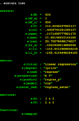
Another class of commands is the eclass commands. The command regress is one of them. If we will run reg, we can then look for saved values with "ereturn list":

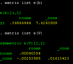
We got the scalars (numbers) that are related to the regression (root MSE, number of observations, F-statistic, R-squared etc.) but also macros (which I personally never use) and most importantly: matrices. One is e(b) which is actually a vector of the coefficients (a matrix of 1 row and 2 columns) , and the other is e(V) which is the coefficients covariance matrix. Let's take a look at them:
And we see, indeed, the coefficients from the regression in e(b). Compare the output of the matrix list e(b) command and the output from the reg command. The e(V) matrix is a bit less self-evident. Remember that the covariance between a variable and itself is its variance. So the coefficient's standard error is actually the square-root of the value it has in the diagonal.
There is, however, a shorter way to reach the coefficient and the standard error. Instead of using the matrices, you can simply refer to the coefficient's value with the _b[] ... thing (I don't know how to call it). In order to get the value of the coefficient of x, put x between the brackets: _b[x] has the coefficient of x from the last regression. So now you can have your program calculate the "effect" of having 3 more rooms and not just one (or just save that number in order to report it in a table later). Also, in order to get the standard error, use _b[]'s brother, which is _se[]. That is:
As long as you didn't run another eclass command, the calculations from the last program will be available for you to use. Once you run the next eclass command (for example, another regression), the saved output will be replaced by the new command's output. The same goes for the rclass commands, but separately. That is, if you run an rclass command, it will not "step on" the eclass command's results, but only the last rclass command's results.
In order to put the results aside for later use (before running the next eclass or rclass command), we will learn how to use macros - in the next chapter.
(Go on to Step #6)


No comments:
Post a Comment