What's so special, really, about the egen (extensions to genereate) command? The answer is that it lets you do lots of things to the data. Things that in other statistical programs might take a lot of commands are possible to do with a couple of egen commands. So this is actually the next phase of data manipulation.
The syntax is pretty simple:
egen <new variable>= <function>(<expression(s)> or <variable(s)>) [, by (<variables>)]
The functions actually determine what the egen command will do. There are many of them, all described in help egen, and the following sectios of this step will describe the use of the most commonly used functions. These examples will hopefully clarify how to use the different functions and how can they help us.
mean()
egen store_mean_price = mean(price), by(store_id)
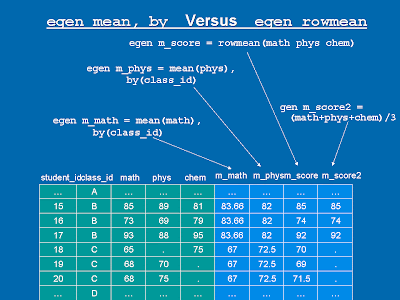
This example will create a variable in which, for each observation, the value will be the mean price of all observations that have the same store_id. See the figure under rowmean() for a graphic illustration.
One can omit the by option - this will put the mean of the original variable for all observations in the dataset.
Other examples:
egen mean_firm_occupation_wage = mean(wage), by(firm_id occupation_id)
This will put, for each observation, the mean wage of all other observatios with the same firm_id and occupation_id.
rowmean()
The function rowmean also compute means, but instead of computing means of a variable across observations, it compute the mean across variables for each of the observations.
egen mean_score = rowmean(math_score physics_score chemistry_score)
Suppose you had a dataset of students and their scores. This example will simply create a new variable - mean_score - which will hold the mean of math, physics and chemistry score for each of the students.
Note that the fact that it computes it separately for each of the observations makes the by option irrelevant. Take the previous example: There's no meaning to do add a by(class_id) option to the egen command when using the rowmeanfunction. If you want the mean score in class for any of the subjects (mean score across students), you should use the mean() function instead of the rowmean(). If you want the mean score (across students) of the mean score (across subjects), you need to first do mean and then rowmean (or vice versa).
You might ask, what's the difference between the rowmean() and simply using the gen command:
gen mean_score = (math_score + physics_score + chemistry_score) / 3
There are two main differences:
1. You can use wildcards - The same rowmean command can be written like this:
egen mean_score = rowmean(*_score)
This is very useful if the list of valiables is very long, or if you think that later on you might add english_score history_score, and so on, to your dataset, and you don't want to update this command every time. To learn more about wildcards, see help varlist.
2. Missing values - If one of the variables mentioned above is missing, gen command will not be able to sum the three variables and will therefore put missing value for mean_score in that observation. This is the case even if the other two scores are not missing. egen rowmean, on the other hand, will disregard the missing values and compute the mean of only the nonmissing values in the variable list. Only if there are missing values in all of the variables specified, egen rowmean will put missing value in the generated variable (just like the gen command). It's up to you to decide which one is better. Sometimes it is enough to have one missing value in order for the mean value to be irrelevant to what you are measuring, and sometimes you may decide that the mean of the nonmissing variables only is good enough.
This slide shows how the mean() and rowmean() functions work:
Note: Although the observations are sorted according to the by variable (class_id) here, it doesn't mean that you should sort them before. egen doesn't need the dataset to be sorted according to the by variable (although I'm guessing that if it's sorted, it will take less time to process).
sum() and rowtotal(), max() and rowmax(), min() and rowmin()
This is the same as mean and rowmean, but instead of calculating means, these functions calculate sums. Here are some examples:
egen team_effort = sum(effort), by(team)
egen total_correct_answers = rowtotal(question_*)
There is a small difference between rowmean and rowtotal in the way missing values are treated. rowtotal simply treats missing values as zeroes. So even if the values are missing in all the specified variables, the new rowtotal variable will be 0. rowmean would have put missing value instead. If you want to put a missing value there, you might want to do something like that:
egen total_correct_answers = rowtotal(question_*)
egen nonmissing_answers = rownonmiss(question_*) // This function puts the number of variables for which this observation had a missing value
replace total_correct_answers = . if nonmissing_answers == 0
drop nonmissing_answers
For max and min, the function gives the maximum or minimum value, respectively, out of all the values of the specified variable (within a group, if you are specifying the by option). Let's say, for example, that you want to normalize all values of the variable wage in a group so that each observation will have 1 if its wage is the maximum wage in a group, 0 if its wage is the minimum and some number between 0 and 1 if it's in between. The following set of commands will do the job pretty easily:
egen max_wage_f = max(wage), by(firm)
egen min_wage_f = min(wage), by(firm)
gen norm_wage_f = (wage - min_wage_f) / (max_wage_f - min_wage_f)
replace norm_wage_f = 0.5 if norm_wage_f == . // This is for the firms in which the maximum wage equals the minimum wage. The command above will give them missing values, because the denominator equals zero
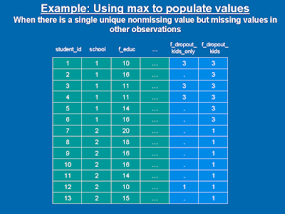
Here is another example of using egen max in order to populate a nonmissing value to observations with missing values. Suppose you have a dataset of students in schools. In one of your regressions you want to take into account the number of children whose father dropped out of high school. In order to do so, you will the following commands:
egen f_dropout_kids_only = count(student_id) if f_educ<12, by(school) // This will count the number of children for whom the condition applies. Observations in which the condition does not apply, will get a missing value to the generated variable.
egen f_dropout_kids = max(f_dropout_kids_only), by(school)
drop f_dropout_kids_only // Don't get confused. This will drop the variable f_dropout_kids_only that is no longer needed
Although, in general, missing value is greater than any other nonmissing value, the egen max ignores missing values and therefore the observations with the nonmissing value in that school - i.e the kids whose father dropped out - will be given to the other observations in the same school (we need all of them in the regression: both the ones who apply and the ones who doesn't). The following figure might make it clearer.
Note: Instead of egen max, we could have also used egen min or egen mean again as the second command. Both egen min and egen mean ignore missing values and since the nonmissing values are equal for that by category, the functions will yield that same value. This is not true for egen sum, though, because the sum function will multiply the nonmissing value by the number of nonmissing observations.
For additional statistical calculations of the within group, see help egen and look for functions such as sd() (for standard deviation), median(), mode() and others. You can also calculate statistics across a group of variables on an observation-basis (instead of across a group of observations on a variable-basis). See help egen and look for the functions that start with row : rowmean(), rowmin(), rowmax(), rowsd(), rowtotal(), etc.
tag() and group()
These two function are really useful with identifying variables that have more than one observation (group-identifying variables) - the same ones we used before in the by options.
Suppose you have a dataset of gas prices. Each observation has the type of fuel, the price per gallon, the station ID, and week in which the price was recorded. Not all stations were recorded in each of the weeks. That is, in some weeks, some stations didn't have their price taken. In your research, you decide to work only on stations for which you have full data - i.e, those which appear in each of the 50 weeks.
If the data had only one observation per station-and-week combination, you could have just used the count() function of egen:
egen station_count = count(week), by(station) // This will count the number of observations with non-missing values in week, for each value of station, and put the result for each observation of that station.
The problem is that each station-week combination has more than one observation and the number of observations per station-week varies between stations (remember, each station-week has as many observations as the number of fuel types - a price for leaded, unleaded, premium, etc.). Simply counting observations will not work here. We need to "tag" stations: in other words, we will create an indicator (a dummy variable) which will be 1 for only one observation per station, and 0 for all other observations of the same station.
Once we tag each new combination of station-week, we can count how many station-week combinations there are for each station -- this will give us the number of weeks for each station. Although I said we need to count, we will use the sum() function of egen, because count() will add to the count observations with 0, whereas sum will not (which is good because we do not want to count the same station-week more than once):
egen station_week_tag = tag(station week) // We're not using the by option since the group-identifying variables are already in the tag.
egen weeks_of_station = sum(station_week_tag), by(station)
Graphically, this is what we actually do:
The group() function is used in the same manner we use the tag() function, but instead of putting 1 in each new combination and 0 in combinations that it has already seen, it puts 1 for all the observations of the first combination it sees, then 2 for all the observations of the second combination, and so on. The benefit of this function is that you can create a full numeric ordered single variable that enumerates all combinations. When we will deal with loops, it might be clearer why this is good.
Conclusion
The egen command can help you play with the data pretty easily and intuitively (once you get the trick of the function you are using). There are other functions of egen I did not describe here. As I said, you can use the help egen, and don't be afraid to experiment with the functions.
To check whether your function work, browse your dataset. Sort it first by the group variables you mentioned, and then just browse the variables you want to. If you have a large dataset, you can limit the browse command using if conditions or in. Here are two examples:
sort firm
browse firm employee wage min_wage_f max_wage_f norm_wage_f in 2000/2200 // This will browse observations #2000 through #2200
browse firm employee wage *_wage_f if firm >= 100 & firm <= 200
You can do the same with the list command, by the way (but list is limited to the width of the output screen).
Good luck!
(Go on to Step #5)


No comments:
Post a Comment